MADS Manual
- Overview and Features
- Execution
- Command-line keywords and options
- Input and output files
- Format of MADS input files
- Compilation
- Verification
- Test examples
MADS (Model Analyses & Decision Support) is an object-oriented code that is capable of performing various types of model analyses, and supporting model-based decision making. The code can be executed under different computational modes, which include (1) sensitivity analysis, (2) model calibration (parameter estimation), (3) uncertainty quantification, (4) model selection, (5) model averaging, and (6) decision analysis.
MADS can be externally coupled with any existing model simulator through integrated modules that read/write input and output files using a set of template and instruction files. MADS can also work with existing control, template and instruction files developed for the code PEST (Doherty 2009).
MADS is internally coupled with a series of built-in analytical simulators (currently the analytical solutions are for contaminant transport in aquifer only). In addition, MADS can be used as a library (toolbox) for internal coupling with any existing object-oriented simulator using object-oriented programming.
MADS provides (1) efficient parallelization, (2) runtime control, restart, and preemptive termination, (3) advanced Latin-Hypercube sampling techniques (including Improved Distributed Sampling), (4) several gradient-based Levenberg-Marquardt optimization methods (including LevMar), (5) advanced single- and multi-objective global optimization methods (including Particle Swarm Optimization, PSO, TRIBES, and SQUADS), and (6) local and global sensitivity and uncertainty analyses (including ABAGUS), and (7) information gap remediation decision analyses (under development).
MADS is written in C/C++ and tested on various Unix platforms (Linux, Mac OS X, Cygwin MS Windows). The MADS simulations are performed using command-line execution. A graphic user interface (GUI) using Java/Eclipse is currently under development as well.
MADS is characterized by several unique features:
- Provides an integrated computational framework for a wide range of model-based analyses, and supports model-based decision making.
- MADS is designed to be capable to work in an adaptive mode with minimum input from the user.
For example, ‘mads s01’ is sufficient to perform calibration of problem ‘s01’ and ‘mads montecarlo s01’ is sufficient to perform uncertainty analysis of problem ‘s01’. All the parameters controlling the performance of these analyses are estimated internally by MADS.
Nevertheless, if needed, the user has the flexibility to specify a wide range of options. - The same problem input file (in the previous case, ‘s01.mads’) is sufficient and can be applied to perform all the possible model analyses supported by MADS.
Different analyses can be invoked using different command-line keywords and options.
If preferred, the keywords can be provided on the first line of the problem input file as well. - Most of the model analysis can be performed using a discretized parameter space (e.g. PPSD, IGPD, ABAGUS).
This can substantially reduce the computational effort to perform various model analyses (e.g. calibration, uncertainty quantification, and sensitivity analysis, performance assessment). - Highly-parameterized inversion where the number of model parameters is substantially greater than the number of model constraints (calibration targets or model observations); a similar approach is called SVD-assist in PEST.
- Permits the use of 'acceptable' calibration ranges for each optimization target.
In this way, the model solutions can be constrained to produce predictions within acceptable calibration ranges.
This feature is implemented using the keyword ‘obsrange’. - Allows the use of an acceptable calibration range for the objective function.
In this way, acceptable model solutions can be identified as those producing objective functions below a predefined cutoff value. Once the objective function is decreased below the cutoff value, the optimization is terminated. This feature is implemented using the keyword ‘cutoff’. - Implements a series of alternative objective functions (OF).
- By default, all the model parameters are internally normalized and transformed in a manner that substantially improves the optimization process.
- Provides the option to perform a series of optimizations with random initial guesses for optimization parameters.
- Provides the option to automatically retry the optimization process using a series of random initial guesses for optimization parameters until an acceptable calibration is achieved (keyword ‘retry’).
- Automatically detects and utilizes multi-processor resources for parallel execution.
- Analyzes the runtime performance of the available parallel hosts (processors); hosts not capable of performing the requested parallel jobs are dynamically ignored.
- Tracks the multiple model files during parallel execution automatically; for the user, there is no difference between serial (using single processor) and parallel modes of execution.
- Performs automatic bookkeeping of all the model results for efficient restart and rerun of MADS jobs (e.g. if the previous job was not completed) and additional posterior analyses.
- Allows the user to perform different types of analyses based on model results stored during previous MADS runs; for example, model runs obtained during model calibration can be utilized in posterior Monte Carlo analyses.
- Provides a built-in protection against simultaneous execution of conflicting MADS runs in the same working directory.
- Automatically renames the files obtained during previous MADS runs by default using unique date & time information in the file names to avoid overwriting.
- Object-oriented design of MADS allows for relatively easy integration with other object-oriented optimization or sampling techniques.
MADS Execution:
mads [ problem_name | input_file_name ] [ keywords | options ]
MADS execution requires at minimum either a problem name (problem_name) or problem input file (input_file_name).
problem name (problem_name): Problem root name defines the file names of various MADS input and outputs files. A problem input file named problem_name.mads is expected to exist.
problem input file (input_file_name): an input file that can completely define the simulated problem. The file follows a predefined MADS format. It includes information about the simulation type, model parameters, and model observations (calibration targets).
The root of the input file defines the problem_name used to specify file names of various files associated with simulation outputs. For example, the file named problem_name.results contains the model results, and the file named problem_name-rerun.mads contains information that allows the last simulation to be restarted with the previous runs calibration results. All the possible model analyses can be performed using the same problem input file (input_file_name).
MADS is compatible to work with PEST control, template and instruction files. To work with PEST files, input_file_name should be a PEST control file problem_name.pst.
After the problem_name or the input_file_name a series of keywords and options can be provided (all optional). All the keywords are case insensitive. If there are no keywords or options, model calibration will be performed by default. The keywords and options can be provided to MADS either on the command-line or on the first line of the problem input file (problem_name.mads).
The keywords and options can be specified in any order; if there are contradictions (for example both ‘montecarlo’ and ‘calibrate’ are provided), the priorities are defined by the keyword order in the problem input file followed by the command-line queue (e.g. the last command-line keyword can overwrite any previous definitions).
Executing MADS without any arguments (‘mads’) produces screen output describing MADS keywords and options for quick reference.
Back to topMADS Command-line keywords and options:
Problem type keywords (all the keywords and options are case insensitive):
forward: Perform a single forward model simulation based on the model parameters provided in the input problem file. The results are stored in a file named problem_name.results.
create: Create a MADS input file with calibration targets based on current model parameters. If the keyword is specified, MADS will perform a single forward model simulation based on the model parameters provided in the input problem file. A file named problem_name-truth.mads is created with the simulated values inserted as calibration target values. The simulation results are stored in a file named problem_name.results.
calibrate: Perform a calibration run where the model parameters are calibrated against the calibration targets. This process can also be called model inversion or parameter estimation. This is the default MADS problem type (if no other problem type keywords are specified). The calibration results are stored in a file named problem_name.results. Calibration can be performed using various optimization techniques (global and local), objective functions, weighting schemes, and optimization constraints. The analyses can be performed using various schemes for computing the initial guesses for optimization parameters. The calibrations can be performed in parallel (available resources are automatically detected) and automatically restarted.
montecarlo: Perform an uncertainty analysis using Monte Carlo sampling. The sampling results are stored in files named (1) problem_name.mcrnd* (including all the Monte Carlo runs), and (2) problem_name.results (representing the result with the lowest objective function). Various alternative sampling techniques can be selected using the keyword ‘smp’. The sample runs can be performed in parallel (available resources are automatically detected) and automatically restarted.
gsens: Perform a global sensitivity analysis. Currently, the Sobol Non-linear Sensitivity method (Sobol. IM, 1993 Global sensitivity indices for nonlinear mathematical models and their Monte Carlo estimates) is implemented. MADS uses Monte Carlo estimation of the Sobol indices, requiring 2 independent random samples with equal dimensions. The number of model evaluations is n * (N + 1) where n is the size of the samples and N is the number of Sobol indices (model parameters). The global sensitivity analysis results are stored in files named problem_name.gsens*.
lsens: Perform a local sensitivity analysis computing the Jacobian matrix either for the initial values provided in the input file or for the final calibration results (depending on the combination of keywords). The local sensitivity analysis results are stored in files named problem_name.sensitivity.
eigen: Perform an eigen analysis of the Jacobian matrix either for the initial values provided in the input file or for the final calibration results (depending on the combination of keywords). The eigen analysis results are stored in files named problem_name.eigen.
abagus: Perform an Agent-Based Global Uncertainty & Sensitivity Analysis (ABAGUS). The ABAGUS run identifies optimization parameter sets producing objective function values below a predefined cutoff value (keyword 'cutoff') or within predefined calibration ranges for each target (keyword 'obsrange') on a discretized parameter space. The ABAGUS results, including optimization parameter values and their associated objective function value are stored in files named problem_name.pssa.
postpua: Perform an analysis of predictive uncertainties (currently processing ABAGUS outputs only; the Monte Carlo outputs will be added in the future). Desired predictions are identified as “observations” with weight>0.
infogap: Perform an information gap decision analysis. Results are stored in files named problem_name-predk.igap, where k is the index of the performance metric prediction (one file is generated for each performance metric prediction). Performance metric predictions are identified in problem_name.mads as “observations” with weight=-1.
Examples for executing different types of model-based analyses with MADS are presented in Examples, Demos, Screenshots, and Comparisons sections.
Back to topCalibration method keywords:
single |
single calibration using initial guesses provided in the input file; |
igrnd |
sequential multi-start (multi-try) calibrations using a set of random initial values; |
igpd |
sequential multi-start (multi-try) calibrations using a set of discretized initial values; |
ppsd |
sequential multi-start (multi-try) calibrations using Partial Parameter Space Discretization (PPSD) method; |
Calibration termination criteria:
eval=[integer] |
terminate calibration if the number of functional evaluations exceeds a predefined value [default eval=5000] |
cutoff=[real] |
terminate calibration (or collect solution in the case of abagus) if the objective function is below the cutoff value [default cutoff=0] |
parerror=[real] |
terminate calibration (or collect solution in the case of abagus) if the estimated model parameters are within a predefined absolute error range from their known true values |
obsrange |
terminate calibration (or collect solution in the case of abagus) if model predictions are within predefined calibration ranges |
obserror=[real] |
terminate calibration (or collect solution in the case of abagus) if model predictions are within within a predefined absolute error range from their observed values |
Calibration options:
retry=[integer] |
number of retries in the case of multi-try (multi-start) model analyses [default retry=0] |
iter=[integer] |
number of Levenberg-Marquardt iterations [default iter=50] |
particles=[integer] |
number of initial particles or tribes [default particles=10+2*sqrt(Number_of_parameters)] |
lmfactor=[double] |
multiplier applied to compute when to initiate LM searches within SQUADS algorithm [default lmfactor=1] |
leigen OR eigen |
eigen analysis of the final optimized solution |
Optimization method (opt=[string]; various combinations are possible, e.g. pso_std_lm_gsl):
opt=lm |
Local Levenberg-Marquardt optimization [default] |
opt=lm_levmar |
Local Levenberg-Marquardt optimization using LevMar library |
opt=lm_gsl |
Local Levenberg-Marquardt optimization using GSL library |
opt=pso |
Global Particle Swarm optimization (default Standard2006) |
opt=apso |
Global Adaptive Particle Swarm optimization (default TRIBES) |
opt=swarm |
Global Particle Swarm optimization Standard2006 (also opt=pso_std) |
opt=tribes |
Global Particle Swarm optimization TRIBES (also opt=pso_tribes) |
opt=squads |
SQUADS: Adaptive hybrid optimization using coupled local and global optimization techniques |
Sampling method (smp=[string] OR mslm=[string] for Multi-Start Levenberg-Marquardt (MSLM) analysis using multiple retries with different random initial guesses for unknown model parameters):
smp=olh |
Optimal Latin Hypercube Sampling [default] (if real = 1 RANDOM; if real > IDLHS; if real > 500 LHS) |
smp=lhs |
Latin Hypercube Sampling (LHS) [default smp=lhs_random] |
smp=lhs_random |
Latin Hypercube Sampling (LHS) with random placement of the particles within hypercube cells |
smp=lhs_center |
Latin Hypercube Sampling (LHS) with particle placement at the center of the hypercube cells |
smp=lhs_edge |
Latin Hypercube Sampling (LHS) with particle placement at the edges of the hypercube cells |
smp=idlhs |
Improved Distributed Latin Hypercube Sampling (IDLHS; aka IHS) |
smp=random |
Random sampling |
Sampling options:
real=[integer] |
number of random realizations (samples) [default real=100] |
case=[integer] |
execute a single case from all the realizations (samples) (applied in PPSD, IGPD, IGRND, MONTECARLO model-based analyses) |
seed=[integer] |
random seed value [randomly generated by default] |
Objective function options:
ssr |
sum of the squared residuals [default] |
ssd0 |
sum of the squared discrepancies |
ssda |
sum of the squared discrepancies and absolute residuals |
ssdr |
sum of the squared discrepancies and squared residuals |
Transformation of parameter space and observations (calibration targets):
nosin |
Sin transformation of optimized parameters is not applied [parameters are sin transformed by default] |
plog=[-1,0,1] |
All (plog=1) or no (plog=0) optimization parameters are log-transformed [default: log transformation is designated for each parameter in the input file (plog=-1)] |
olog=[-1,0,1] |
All (olog=1) or no (olog=0) observations (simulated and measured) are log-transformed [default: log transformation is designated for each observation in the input file (olog=-1)] |
oweight=[-1,0,1,2] |
Weights for all the observation residuals in problem_name.mads are overwritten: 0 = zero weight, 1 = unit weight, 2 = weight inversely proportional to observation [default: designated weights in problem_name.mads are used (oweight=-1)] |
Parallelization:
np=[integer] |
number of requested parallel jobs [optional] |
rstfile=[string] |
name of existing zip restart file to be used (created by previous Parallel MADS run) [optional] |
restart=[integer] |
restart=1 (default; automatic restart if possible); restart=0 (force no restart); restart=2 (force restart); by default the analyses will be restarted automatically (restart=1) |
ABAGUS (Agent-Based Global Uncertainty & Sensitivity Analysis) options (abagus):
infile=[string] |
name of previous ABAGUS results file to be used to initialize KD-tree [default=NULL] |
energy=[integer] |
initial energy for swarm [default energy=10000] |
cutoff=[real] |
maximum objective function value for acceptable solutions to be collected |
obsrange |
collect solutions that produce simulations within predefined calibration ranges for each target |
Information gap decision analysis options (infogap):
infile=[string] |
name of ABAGUS results file to perform information gap decision analysis |
Predictive uncertainty analysis options (postpua):
infile=[string] |
name of ABAGUS results file to perform predictive uncertainty analysis |
Build-in analytical solutions:
point |
point contaminant source in 3D flow domain |
plane |
areal contaminant source in 3D flow domain |
box |
block contaminant source in 3D flow domain |
Built-in test problems for global optimization / uncertainty-quantification techniques (local techniques will not work):
test=[integer] |
test problem ID [default=1]: Curve-fitting test functions: |
dim=[integer] |
dimensionality of parameter space for the test problem (fixed for some of the problems) [default=2] |
npar=[integer] |
number of model parameters for the data fitting (fixed for some of the problems) [default=2] |
nobs=[integer] |
number of observations for the data fitting test problem (fixed for some of the problems) [default=2] |
pardomain=[float] |
parameter space domain size [default pardomain=100] |
Debugging / verbose levels:
debug=[0-5] |
general debugging [default debug=0] |
fdebug=[0-5] |
model evaluation debugging [default fdebug=0] |
ldebug=[0-3] |
Levenberg-Marquardt (LM) optimization debugging [default ldebug=0] |
pdebug=[0-3] |
Particle Swarm optimization debugging [default pdebug=0] |
mdebug=[0-3] |
Random sampling debugging [default mdebug=0] |
odebug=[0-1] |
Objective function progress [default odebug=0] |
tpldebug=[0-3] |
Debug the writing of external files [default tpldebug=0] |
insdebug=[0-3] |
Debug the reading of external files [default insdebug=0] |
pardebug=[0-3] |
Debug the parallel execution [default pardebug=0] |
MADS Input and output files
problem_name.mads: an input file that can completely define the analyzed problem. The file follows a predefined MADS input format. It includes information about the simulation type, model parameters, and model observations.
problem_name.results: an output file containing the MADS results
problem_name.residuals: an output file containing the residuals between model predictions and calibration targets (if applicable)
problem_name.jacobian: an output file containing the Jacobian (local sensitivity) matrix
problem_name.covariance: an output file containing the covariance matrix
problem_name.correlation: an output file containing the correlation matrix
problem_name.eigen: an output file containing the eigen matrix and eigen values
problem_name.phi: an output file containing information about the final objective function
problem_name.ofe: an output file containing information about the objective function minimization progress as a function of model evaluations
problem_name.mcrnd*: output files containing Monte Carlo (MC) analysis results
problem_name.igrnd*: output files containing Random Initial Guesses (IGRND) results
problem_name.igpd*: output files containing Partially Discretized Initial Guesses (IGPD) results
problem_name.ppsd*: output files containing Partial Parameter Space Discretization (PPSD) results
problem_name-rerun.mads: an output file that can be used as a MADS input file. It contains all the information needed to restart the last calibration. The model parameters are modified to represent the current best estimates. The file follows a predefined MADS input format.
problem_name.igap: output files containing remediation information gap (infogap) results
problem_name.pssa: output files containing ABAGUS results
problem_name.pua: output files containing predictive uncertainty analysis (postpua) results
Format of MADS input files
MADS Problem files (*.mads)
The MADS input problem files provide information about the model parameters needed to execute the model simulator and the model observations (calibration targets) that will be applied to evaluate the model performance. The input file typically has the following format (this example file called w01.mads is located in directory example/wells-short):
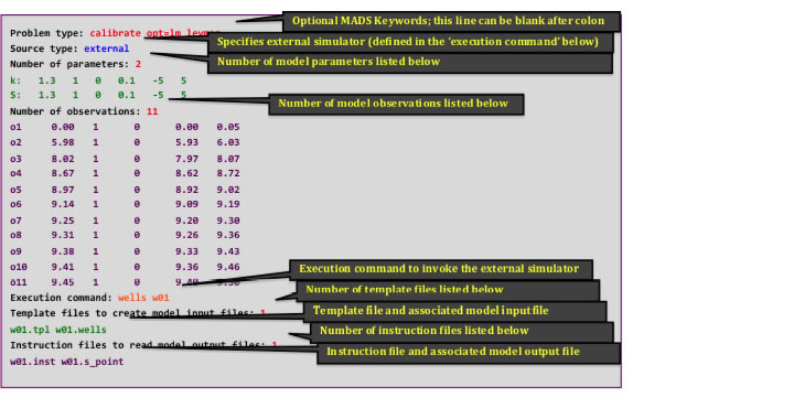 [click to enlarge]
The key data blocks in the MADS problem file are defined above.
The format associated with model parameters and observations is defined below.
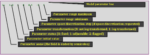 [click to enlarge]
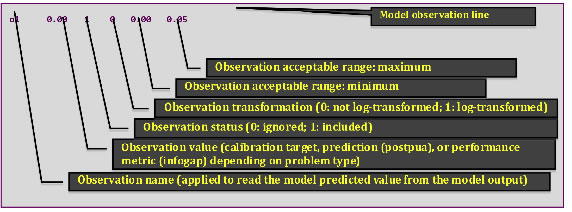 [click to enlarge]
Instead of MADS problem file, MADS can also read and work with the standard PEST control (problem) files (‘*.pst’) without any conversion.
MADS Template files (*.tpl)
The MADS template files provide the current values of the model parameters to the external simulator. In this case, the file ‘w01.tpl’ is applied to create the model input file ‘w01.wells’. The file ‘w01.tpl’ is located in directory ‘example/wells-short’. The template input file typically has the following format:
 [click to enlarge]
In this case, the template file is based on the WELLS (wells.lanl.gov) input file where two of the input model parameters (‘Permeability’ and ‘Storage coefficient’) will be replaced by MADS with the current values associated with these model parameters. The model parameters are defined in the MADS problem file ‘w01.mads’ and labeled as “k” and “S”. The first line with the keyword ‘template’ is optional. In this case, it defines the special variable symbol “%” that is going to be applied to define the fields where model parameters will be placed. If the first line is missing, the special variable symbol “#” is assumed by default. More than one template files can be applied to generate a series of model input files. Each model parameter can appear multiple times in the template files.
The easiest way to create a template file is to take an existing model input file and replace the model parameters provided to MADS for analysis with the name of model parameters as defined in the MADS problem file. The model parameter names should be surrounded with the special variable symbol.
The MADS template file format is similar to the format implemented in the code PEST. In fact, MADS can use the standard PEST template files as well without any conversion.
The template files can be debugged using the keyword ‘tpldebug’ (for example:‘mads w01 tbldebug’).
MADS Instruction files (*.inst)
The MADS instruction files are applied to read the current model observations (predictions) obtained from the external simulator based on the current model parameters. In this case, the file ‘w01.inst’ is applied to read the model output file ‘w01.s_point’. There are several alternative versions of the instruction file (‘w01-v*.inst’) provided in directory ‘example/wells-short’. The instruction files typically have the following format:
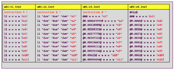 [click to enlarge]
The observation names are shown in ‘red’ and are specified in the MADS control file. All the instruction files presented above are equivalent in terms that all of them are extracting the same information from the model output file ‘w01.s_point’. The file format is somewhat similar to the format implemented in the code PEST. In fact, MADS can use the standard PEST instruction files as well without any conversion.
The first line with the keyword ‘instruction’ is optional. In the case of ‘w01-v1.inst’, it defines that the special search symbol “%” is going to be applied to search for numeric or character patterns in the model output file, the special observation symbol “!” is going to be applied to define the location of the observations within the model output file. If the first line is missing as in the case of ‘w01-v4.inst’, the symbols “@” and “!” are assumed by default for the search and observation tokens, respectively. Each consecutive instruction line in the instruction file starts with either (1) the letter “l” or (2) the special search symbol. In the case of “l”, the following number defines how many lines to be skipped (for example, “l1” means go to the next line; “l2” means skip one line). In the case of search symbol, the content of the model output file is skipped until search phrase is found. The letter “w” forces skipping of white-character spaces. The keyword “dum” defines dummy observations that are ignored.
Note that the search phrase “@0@” in files ‘w01-v3.inst’ and ‘w01-v4.inst’ can be dangerous since the digit “0” can occur in many locations in the model output file.
Comparing ‘w01-v3.inst’ and ‘w01-v4.inst’ it is clear that the search pattern does not need to include the entire number of characters that are expected to be in the model output file. The search pattern also does not need to be at the beginning of the line.
The instruction files can be debugged using the keyword ‘insdebug’ (for example: ‘mads w01 insdebug’).
MADS Compilation
To compile, extract the provided mads.tgz file (tar xvf mads.tgz) and execute 'make'. GSL, LAPACK and BLAS libraries are expected to be available.
- GSL: ftp://ftp.gnu.org/gnu/gsl/
- LAPACK: http://www.netlib.org/lapack/
- BLAS: http://www.netlib.org/blas/
If macports is installed (www.macports.org), these packages can be installed on MAC OS X machines using the following commands (requiring administrative privileges):
- sudo port install blas
- sudo port install lapack
- sudo port install gsl
MADS Verification
To verify that MADS is running properly, execute 'make verify'.
MADS Test Examples
To run some of the available MADS examples, execute 'make examples'.
Back to top